This post is a quick intro to overtones, harmonics and additive synthesis, using a video lovingly prepared by Synth School as a reference point:

These are the building blocks of synthetic computer sound, so it pays to spend some time getting a grasp of the basics.

The two views: Oscilloscope vs. Frequency Analysis
One of the first things in the video is a comparison of the representation of a sine wave in an oscilloscope, against a sine wave in a frequency analysis view:

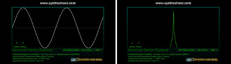
This is useful, because if you are working with computer sound, these two views are like bread and butter (or perhaps rice and water, depending on your preferred diet).

Sampling and the Oscilloscope view
In any short period of digitally recorded audio, say one second, we can store a number of samples, i.e. numbers between -1 and +1, to represent the movement of a loudspeaker during that time. We say that any given sample within our set of samples will have an amplitude value between -1 and +1.

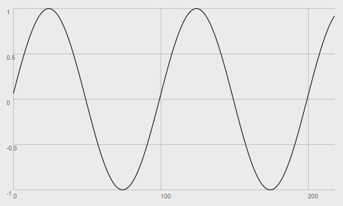
In the Oscilloscope view, we lay out the samples over time (X axis), with earlier samples on the left and later samples on the right. We lay out the amplitude values on the Y axis, with 0 in the middle, +1 at the top, and -1 at the bottom.

The amplitude of any sample at any moment in time represents whether our loudspeaker will be 'sucked in' at that moment (somewhere between -1 and 0), or 'pushed outward' (somewhere between 0 and +1), or at rest (exactly 0). Note that numbers lower than -1 or higher than +1 will either be 'clipped', or will damage our loudspeakers.

So as we 'read' the Oscilloscope view left-to-right, we read the history of the loudspeaker's movements in detail. This is great, but this only tells one part of the story - the very literal part. The next part of the story - frequency analysis - is more abstract, but much more powerful in the information it can reveal.

But first, something very important, very quickly - sample rates.

The sample rate
In the Oscilloscope image above there are just over 200 samples represented. All this tells us is that there are 200 samples - it doesn't tell us over what period of time. To know that, we need to know our sample rate - the number of samples we have chosen to store per second.

If we have a sample rate of 200, then 200 samples will represent one second. In reality, we need far higher sample rates for our ears to think of all those samples as a continuous stream rather than as a series of individual sounds. For example, 44,100 samples per second is a common standard.

That's all I'll say for now - it just pays to introduce the idea while we are already looking at samples anyway in the Oscilloscope view.

The Frequency Analysis view
If the Oscilloscope view gives us a very literal perspective of a waveform - simply it's linear changes over time - what does frequency analysis give us?

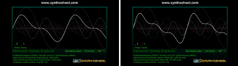
As the Synth School video demonstrates so eloquently, we can combine certain periodic waveforms, such as sine waves, to create fuller-bodied, often more harmonically resonant sounds. If we can use multiple simple waves at readable frequencies to construct a sound, surely we can reverse the process, and de-construct said sound into constituent frequencies...

This is the idea behind Fast-Fourier Transform (FFT), and FFT is the algorithm that takes a series of samples (like the one we used to make our Oscilloscope view) and builds a graph showing which frequencies are present in those samples.

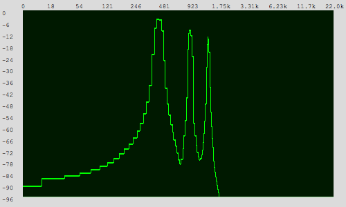
In fact, the Frequency Analysis view is just the visual result of running the FFT algorithm, so you will often hear it called the FFT view. In the FFT view, volume is on the Y axis (from -96dB to 0dB) and frequency is on the X axis (depending on your readout this will plot 0 times per second all the way to 22,000 times per second - aka 0Hz to 22kHz). So you can think of the FFT view as giving you the relative amounts for each frequency in your set of samples.

Looking at the X axis more closely, you'll notice that half of the scale is dominated by frequencies in the early hundreds. Zero to 923 take up over half the scale, and 923 to 22,000 get less than half! That's just because of the way we are visualizing it.

It's a logarithmic scale because in most practical scenarios most of the action takes place on the left-hand side of the scale, and a logarithmic scale helps us get a better view of that action. However, most FFT views have the option of switching to a linear scale view, and then you will see most of the action taking place on the far left of the view.

Fundamental and overtones
A sine wave is often called the only 'pure' tone because it is the only waveform type to contain only a single frequency, as we saw in the Synth School video. This frequency is called the fundamental.

Other waves always have additional frequencies on top of the fundamental. The lowest frequency of the sound, the fundamental, is the basic tone on which the sound is built. Additional frequencies are called overtones. The fundamental and it's overtones are collectively called partials.

Overtones can be harmonic, or inharmonic. Harmonic overtones support the fundamental frequency and keep it's tonality intact. Non-harmonic overtones result in noise, or sounds with ambiguous pitch.

However it is the relationship between a fundamental and it's overtones, and the relationship of the overtones to each other that make up the sound's timbre - it's unique characteristic audible effect. Acoustic instruments have lots of complex activity in non-harmonic overtones. They are generally not loud enough to undermine the fundamental, but are loud enough to add character to the sound.

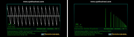
Additive synthesis
A saw wave can be constructed by combining multiple sine waves, as demonstrated in the video. For a 'classic' saw tone, the amplitude of each added harmonic should be divided by it's harmonic count, i.e. the fundamental is divided by 1, the second harmonic is divided by 2, the third by 3 and so on.

So a saw tone can be thought of as the combination of infinite harmonics, each divided by the harmonic count. Though in practice doing so would require infinite CPU power!

Square wave
A square wave is also constructed by adding harmonics, but this time only odd-numbered harmonics, i.e. by skipping the 2nd, 4th, 6th (etc) harmonics, and including those in between.

This is illustrated quite nicely in this old-school training video:

That's a nice intro to overtones, harmonics and additive synthesis. For more on hands-on additive synthesis and beyond, I recommend Welsh's Synthesizer Cookbook.